ResearchTraceDB
TraceDB: a database for what happened next
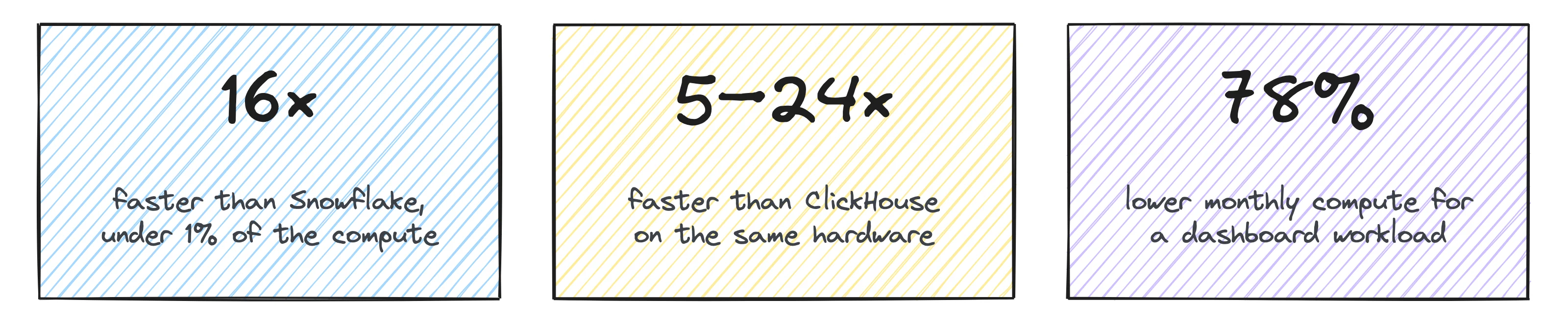
Your warehouse is great at totals. Ask it what happened next (after a failed tool call, before a cancellation, between “pending” and “shipped”) and it grinds. TraceDB is built for exactly those questions: 16× faster than Snowflake for under 1% of the compute, and 5–24× faster than ClickHouse on the same hardware.

What TraceDB is for
Questions about event data come in two flavours.
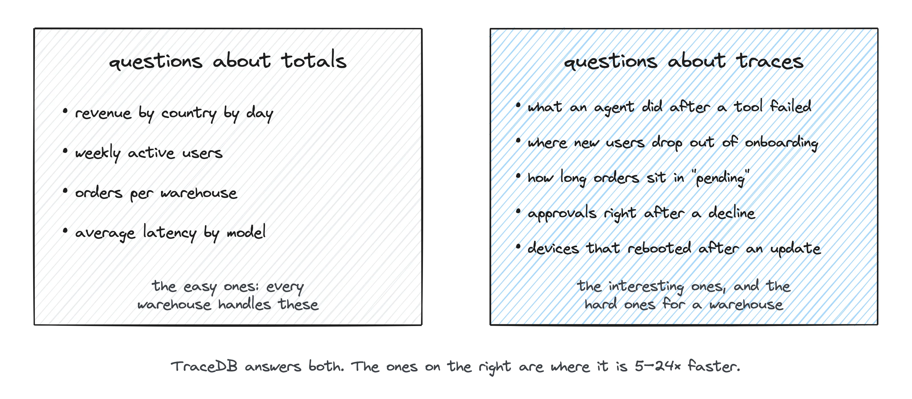
The first kind is about totals: revenue by country, weekly active users, orders per warehouse, average latency by model. These are the easy ones. Every warehouse handles them well, and TraceDB can answer them too, but it won’t be much faster.
The second kind follows one thing through time: a user, an order, a device, an agent run. We call these trace questions, and they’re where things get interesting. What does an agent do in the three steps after a tool fails? Where do new users drop out of onboarding, and what were they doing right before? How long does an order sit in “pending payment” before it ships? Which card approvals came minutes after a decline? Which devices rebooted right after a firmware update? These are usually the questions you actually care about, and they’re the ones that turn into a 40-line query, a stalled dashboard, or a ticket for the data team. To answer any of them, a database has to follow each user, order, card or device through time, one event after the next.
Warehouses aren’t set up for that. They lay events out for scanning columns, usually partitioned by date and sometimes clustered on a key or two. That’s ideal for totals, but it means one user’s (or order’s, or device’s) events end up spread across every partition in the date range. So every trace question starts with the same chore: read all of it, group the rows by user, sort each group by time, and only then work out the answer. Even if you sort the table by user, as you can in ClickHouse, the query still rebuilds each history with window functions and self-joins. Ask a follow-up and it does the whole thing again.
TraceDB skips the chore. It keeps each one’s events together, in order, from the moment they land. We call that ordered history a trace.1 The gathering and sorting is already done, so every question goes straight to the part you asked about.
This matters even more once agents start asking. A person might glance at a dashboard of totals and move on. An agent asked “why?” tends to go straight for trace questions: who did this, what did they do first, what happened right before, how are they different from everyone else. And it asks them back to back, each one about the same group as the last.
(A trace can belong to whatever your events are about: a user, an account, a device, a card, an agent run, or a row in a table that keeps changing. Below we’ll say “customer” to keep things short.)
Use cases
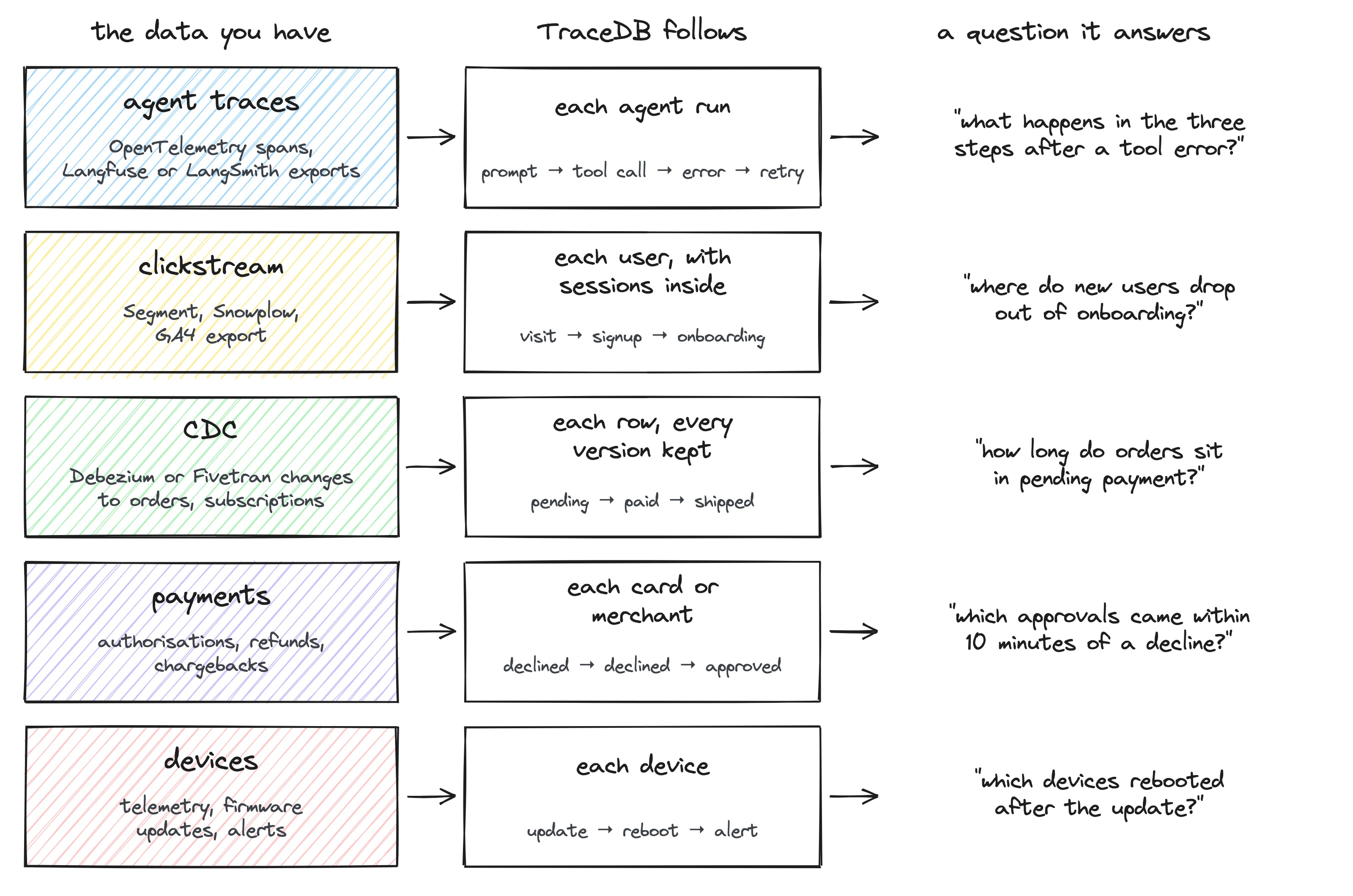
Trace questions show up anywhere the same thing happens to someone, or something, more than once. Chances are you already have this data sitting in your warehouse, in one of a few shapes, and you won’t need to reshape any of it: TraceDB maps your existing tables onto traces for you.
Agent traces
The data: if you run an AI product, you’re probably logging every step your agents take, as OpenTelemetry spans or exports from Langfuse, LangSmith or your own logging. Each row has a run or conversation ID, the step (prompt, model call, tool call, tool result, error), the tool and model, latency, tokens and status.
TraceDB follows each agent run, so every run is one trace, in order. You can follow whole conversations or users the same way.
The kind of thing you’d ask:
- What happens in the three steps after a tool error: a retry, a different tool, or a give-up?
- Which runs called the same tool again within a minute of it failing, and which tools does that happen to most?
- Did ratings drop for runs that hit the failing tool, compared with runs on the same app version that didn’t?
- How many tokens does a resolved conversation cost, against one that ends without an answer?
-- runs that called a tool again within a minute of an error, by tool
SELECT tool, count(DISTINCT entity) AS runs
FROM events
WHERE event = 'tool_call' AND preceded_by('tool_error', '1m')
GROUP BY tool
ORDER BY runs DESC
Most observability tools are great at showing you one trace. They get a lot less helpful when you want to ask something across a million of them. That’s the gap here. The benchmark data later in this post has exactly this shape, and on “what followed each tool error” over a billion events, TraceDB was 24× faster than ClickHouse.
Clickstream and product analytics
The data: page views, clicks and tracked events from Segment or RudderStack, Snowplow’s atomic events, the GA4 export, or Amplitude and Mixpanel exports. Usually one big, wide table with a user ID, an anonymous ID, an event name, a timestamp and a bag of properties.
TraceDB follows each user, and finds their sessions inside the trace. Visitors usually start out anonymous. If you keep a table that maps anonymous IDs to users, TraceDB follows that too, and moves a visitor’s earlier events onto their trace once they sign up.
Questions it answers:
- Where do new users drop out of onboarding, by platform, within their first week?
- How do sessions open, and what do people do in the 10 minutes before they buy?
- How long from signup to first purchase, and does it differ by acquisition channel?
- Of the users who came back in week 4, what did they do in week 1 that the others didn’t?
-- signup to first project within a week, by platform
SELECT *
FROM funnel('signup', 'onboarding_done', 'first_project',
            window => '7d', group_by => 'platform')
If this list sounds like Amplitude or Mixpanel, that’s the point: the same questions, asked of the events already in your warehouse, without shipping a copy off to another vendor. On “how sessions open” over a billion events, TraceDB was 22× faster than ClickHouse.
CDC, payments, devices: same idea
Once you see the pattern, it shows up everywhere. Pick the thing you care about, follow its events in order, and the same few questions come up: what came before, what came after, how long in between, and what was true at the time.
- CDC tables (Debezium, Fivetran or Airbyte syncs of
orders,subscriptions,tickets). Each row becomes a trace, and every change TraceDB sees stays on it, even after the warehouse overwrites the old value. “How long do orders sit in pending payment?” and “which plan was the account on when the ticket opened?” stop being as-of joins against a history table nobody kept. - Payments. Each card or merchant is a trace of authorisations, refunds and chargebacks. Most fraud rules are really trace rules, like an approval within 10 minutes of a decline, and they tend to be the ugliest SQL in the building.
- Devices. Each device is a trace of readings, updates, reboots and alerts. Its firmware version holds until it changes, so “which devices rebooted within 10 minutes of an update, by firmware?” is one filter.
Agents asking questions about any of these
This one isn’t a kind of data. It’s a kind of user. Hand an agent any of the data above and ask it something open-ended, like “why did cancellations jump last week?”, and its next dozen queries map neatly onto the patterns in this post:
| The agent asks | The pattern | In TraceDB |
|---|---|---|
| Who cancelled within five days of signing up? | something that happened within a window after something else | followed_by('cancelled', '5d') on each signup |
| Which plan were they on when they signed up? | a value as it was at a moment | plan on the signup event |
| What did they do in the hour before cancelling? | what came right before | followed_by('cancelled', '1h') |
| How are they different from the ones who stayed? | the same group, compared with everyone else | a saved group: in_cohort('early_cancellers') |
| Show me a few of them, start to finish. | one customer’s whole history | WHERE entity = '…' ORDER BY ts |
Every step is a trace question, and every step after the first is about the same group of customers. That’s why TraceDB lets an agent save a group once and have each follow-up read only those customers. Agents aren’t the biggest source of queries on most warehouses today, but this is how they use data when they do, and it’s the workload we originally built TraceDB for. There’s more on how it plays out in practice below.
Beside your warehouse
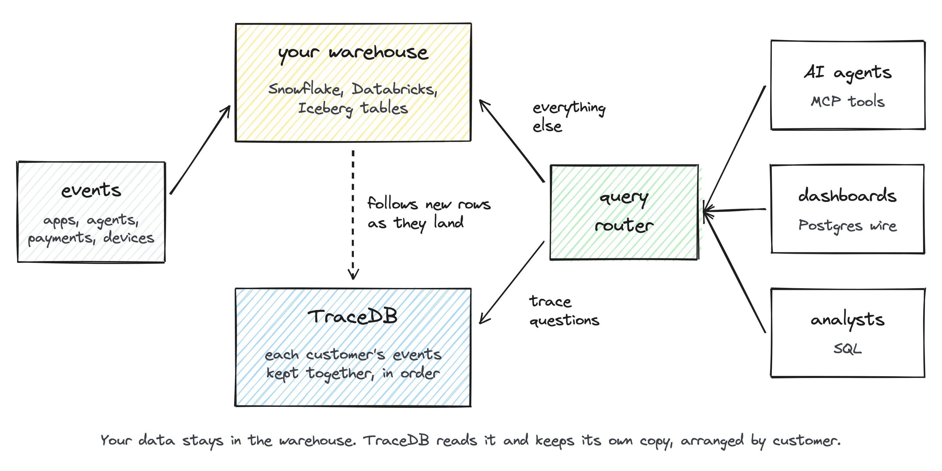
You don’t have to move or reshape anything. Point Embrasure at the tables you already have (lakehouse event tables, CDC tables, plain dimension tables) and it works out the mapping on its own: which column says who a row is about, which one is the time, and which columns are events versus attributes that change over time. TraceDB builds the traces from that and keeps up as new rows land. You can look over the mapping and fix anything it got wrong. Your pipelines, dbt models and dashboards stay where they are, and the warehouse stays the source of truth.
There are three ways in:
- AI agents use MCP tools with a query language built around customers and saved groups of them.
- Dashboards and BI tools connect over the Postgres wire protocol, like any Postgres database.
- Analysts write SQL: standard SQL plus a few functions for traces, such as
paths(),occurrence(),followed_by(),sessions()andfunnel().
A query router sits in front of both. Trace questions go to TraceDB, everything else goes to the warehouse, and nobody has to think about which is which. If TraceDB can’t answer something, the warehouse picks it up.
One question, two SQLs
Here’s what the difference looks like. Say you want to know what happened right after each tool error. In TraceDB, that’s:
TraceDB
SELECT path, count, entities
FROM paths(from => 'tool_error', steps => 2)
ORDER BY count DESC
LIMIT 10
The same thing in standard SQL (ClickHouse, Snowflake, most warehouses)
SELECT concat(event, ' → ', next_1, ' → ', next_2) AS path,
  count(*) AS count, count(DISTINCT user_id) AS entities
FROM (
  SELECT user_id, event,
    lead(event, 1, '(end)') OVER w AS next_1,
    lead(event, 2, '(end)') OVER w AS next_2
  FROM events
  WINDOW w AS (PARTITION BY user_id ORDER BY ts)
) t
WHERE event = 'tool_error'
GROUP BY path
ORDER BY count DESC
LIMIT 10
Same ten rows back. The second one sorts every user’s whole month of events to find the two that come after each error. TraceDB reads them straight off each trace.
One more: what did buyers do in the 10 minutes before a purchase?
TraceDB
SELECT event, count(*) AS events,
  count(DISTINCT user_id) AS users
FROM events
WHERE followed_by('purchase', '10m')
GROUP BY event
ORDER BY events DESC
Standard SQL: a self-join
SELECT e.event, count(*) AS events,
  count(DISTINCT e.user_id) AS users
FROM events AS e
JOIN (SELECT user_id, ts AS bought
      FROM events WHERE event = 'purchase') AS p
  ON e.user_id = p.user_id
WHERE e.ts < p.bought
  AND e.ts > p.bought - INTERVAL '10 minutes'
GROUP BY e.event
ORDER BY events DESC
It’s the same story across the usual trace questions:
| You want | TraceDB SQL | Standard SQL |
|---|---|---|
| what came next | paths(from => 'tool_error', steps => 2) | lead() over each user’s events, sorted by time |
| each user’s first purchase | occurrence('purchase') = 1 | row_number() per user, or ClickHouse’s LIMIT 1 BY |
| events shortly before a purchase | followed_by('purchase', '10m') | a self-join on user and a time range |
| sessions | sessions() | lag() to find the gaps, then a running sum |
| a funnel | funnel(...) | one self-join per step, or ClickHouse’s windowFunnel |
Shorter SQL is nice, but the real win is fewer mistakes. Every self-join and window function is another place for an analyst, or an agent, to get a detail subtly wrong, like counting customers whose five days aren’t up yet as “didn’t cancel.” The query runs fine. The answer is a little off. Nobody notices.
TraceDB and Snowflake
Let’s start with Snowflake, since that’s where a lot of event data already lives.
We loaded the same 100 million synthetic events (a month of an AI product’s telemetry, with an incident planted in it)2 into both. Then we had each engine answer the six questions an agent asks while investigating that incident: how the failing calls break down by app version, what users did after a failure, how their sessions went, which users hit the failure at least twice, how those users rated the product, and how far they got through the main funnel. TraceDB ran on four cores of an AWS Graviton machine. Both got all six answers exactly the same.
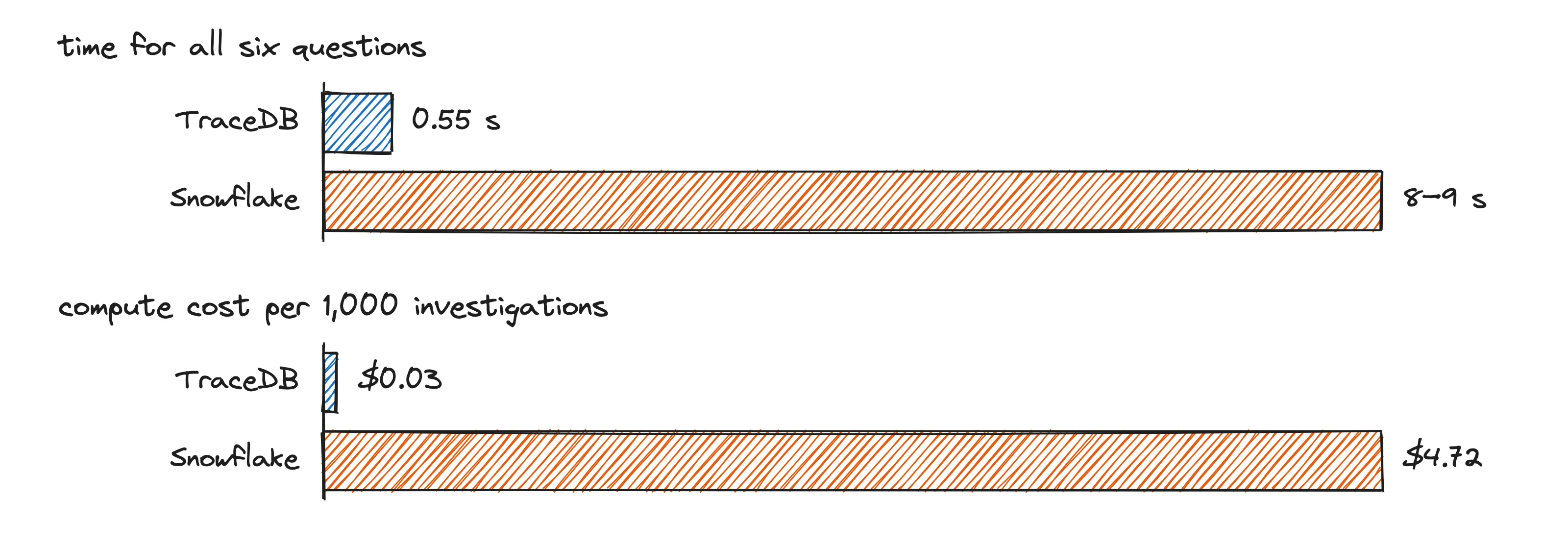
TraceDB finished all six in 0.55 seconds. Snowflake took 8 to 9. You could throw a bigger warehouse at it, but each size up doubles the credits per hour, so you’re paying about the same per question to get there faster.
Now the money. At $2 a credit,3 8.5 seconds of Snowflake is about half a cent, or $4.72 per thousand investigations. TraceDB’s 0.55 seconds on an m8g.xlarge (about $0.18 an hour on demand) comes to 3 cents per thousand. That’s compute per question, though, and real bills are messier: you also pay for TraceDB’s machines while they sit idle, and for whatever still goes to Snowflake.
So we tried a more realistic bill. We replayed a dashboard workload through the router: a Superset dashboard over the same events, opened and explored the way people do, including a few window-function queries the router sent back to Snowflake. The dashboard opened in 1.3 seconds instead of 2.5, every tile matched, and at 1.5 million queries a month the projected compute fell from $1,481 to $327, with two always-on TraceDB machines counted in.
| Workload | TraceDB | Snowflake |
|---|---|---|
| Agent investigation: 6 questions, 100M events | 0.55 s | 8–9 s |
| Compute per 1,000 investigations | $0.03 | $4.72 |
| Dashboard open in Superset, incident week | 1.3 s | 2.5 s |
| Dashboard workload, 1.5M queries a month (projected) | $327 a month, including two always-on machines | $1,481 a month |
| Plain totals over the whole month | about 1.5× faster | close behind |
Keep an eye on that last row. For plain totals over a long range, Snowflake’s fixed overhead per query is a small part of the time, and the gap shrinks to about 1.5×. The big wins are on trace questions, and on the short, frequent queries that dashboards and agents fire off all day.
TraceDB and ClickHouse
ClickHouse is the tougher opponent. It’s the fastest open-source analytics engine most teams know, and it’s usually what people reach for when Snowflake gets too slow or too expensive for event data.
So we gave it every chance to win. Both engines got identical machines (4 cores, 16 GB) with their data in S3 and a local cache, over the same billion events. ClickHouse got two copies of the table, one partitioned by day and one sorted by user, and we counted whichever was faster for each question. Its SQL was the fastest we could write, including hand-tuned per-user arrays that run about 3× faster than the window functions shown above. Every answer matched.
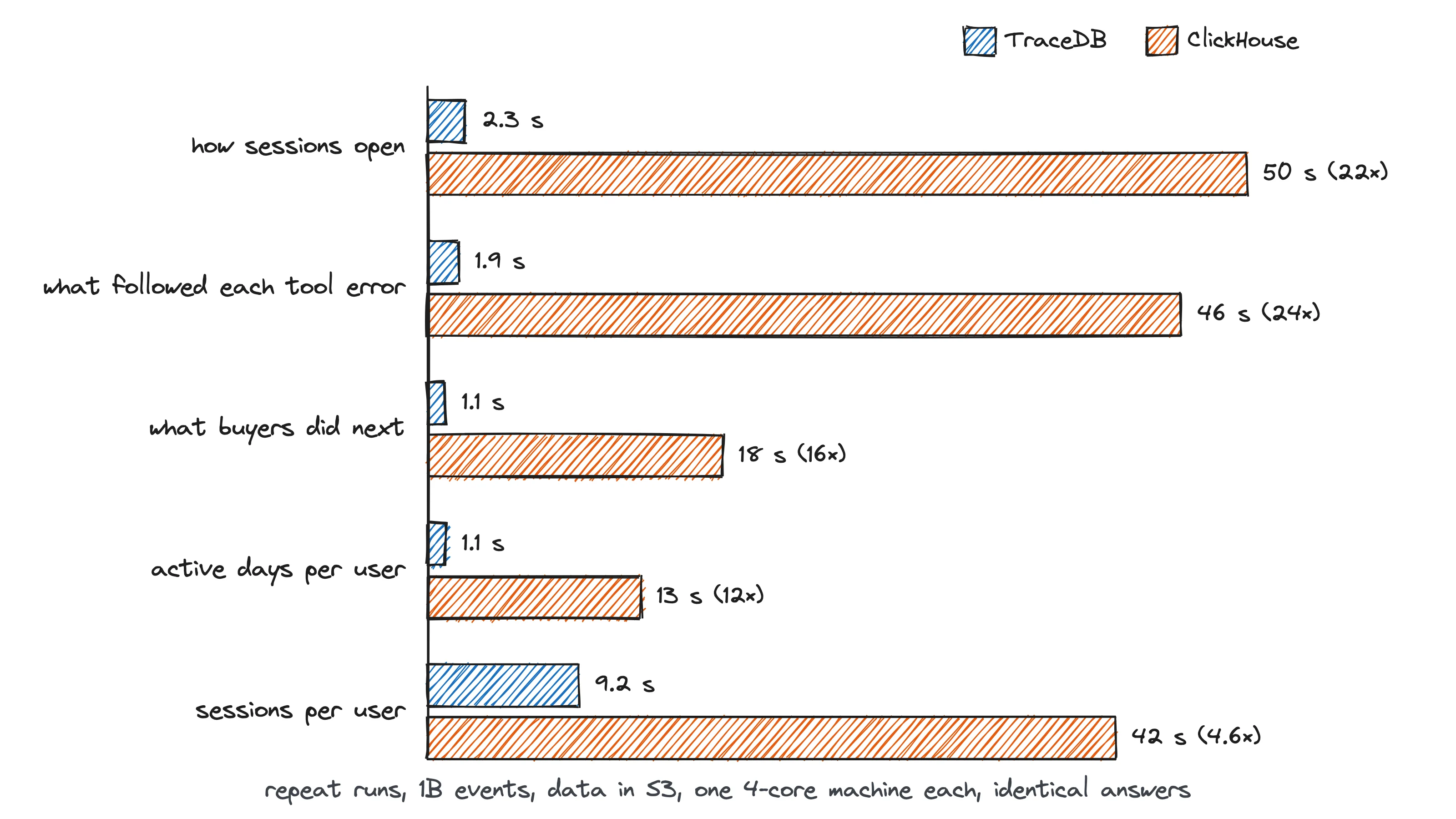
On repeat runs, TraceDB was 5 to 24× faster. The first run after a restart, with everything pulled from S3, is closer: about 4× at 100 million events, and 1.9× on the closest question.
Same machines, so cost per question tracks time: a twentieth of the time is a twentieth of the machine. There’s another cost that’s easy to miss. The fast ClickHouse SQL for these questions packs each user’s events into arrays of integer codes, and it takes someone who really knows ClickHouse to write and maintain it. The plain window-function version is another 3× slower. With TraceDB, the fast version is also the short one.
To be fair to ClickHouse, it wins some questions too. They’re not in the chart because the chart is about the questions TraceDB is built for, so here they are:
- looking up one user’s events, which ClickHouse answers in about 10 ms;
- filtering events by a list of users computed in a subquery (0.6 s against TraceDB’s 1 s);
- “A followed by B within an hour”, where the two are even or ClickHouse is ahead.
What it changes for AI agents
For agents, query speed is only part of the story. Most of what an agent costs is model turns, and every failed query, or step spent rebuilding the same group of customers, is another turn.
We ran Embrasure’s own data agent over three benchmark datasets (product analytics, a ledger, and a dbt project) two ways: TraceDB first, or warehouse SQL only. Same model, same prompts, same questions.4
| Dataset | TraceDB first | Warehouse SQL only |
|---|---|---|
| Product analytics: correct, median time | 116/120, 17 s | 120/120, 30 s |
| Ledger: correct, median time | 118/120, 30 s | 110/120, 35 s |
| dbt project: correct, median time | 87/90, 18 s | 84/90, 27 s |
| Cost per correct answer (product, dbt) | $0.29, $0.30 | $0.35, $0.36 |
With TraceDB the agent was faster on every dataset, and at least as accurate on two of the three. We’ve since fixed the misses on the first one, and the latest runs score 30 out of 30 on all three.
Two things do most of the work. First, an agent can save any answer as a named group of customers and ask follow-ups about just that group: on 250 million events, a breakdown of a 9,228-account group takes 4 ms. Second, TraceDB tells you when it doesn’t know. A customer whose five days aren’t up yet comes back as unknown instead of “no”, so the agent doesn’t build on a quiet mistake.
How it works, briefly
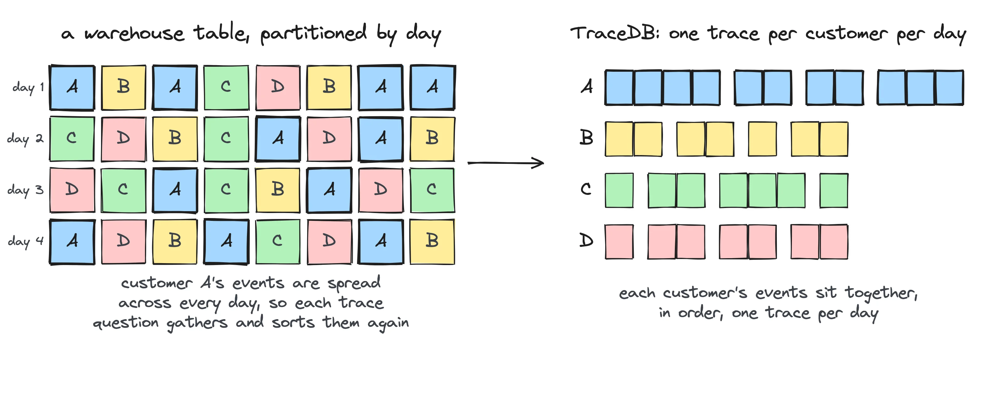
The short version: TraceDB stores events by customer and by time period: each customer’s events from each day (or hour, or week) are kept together as one trace. Its indexes point at traces, so a question about a rare event reads only the traces that contain it. Attributes such as a customer’s plan are tracked as they change, so “plan at signup” is a lookup instead of a join. New events can be queried as soon as they arrive. And because customers are independent of one another, TraceDB spreads across machines by customer.
What stays in the warehouse
TraceDB isn’t meant to do everything, and that’s fine. The router sends these to the warehouse so you don’t have to think about it:
- Plain totals over whole tables. Columnar warehouses are as fast, or close.
- Joins between different kinds of thing, like orders and the support agents who handled them. TraceDB follows one kind of entity at a time; these go to the warehouse.
- Single-record lookups, where ClickHouse and most warehouses are already quick.
- The source of truth. TraceDB keeps a copy shaped for trace questions. Your warehouse keeps the data.
Getting started
TraceDB runs inside Embrasure. Connect your warehouse and pick your event tables. Embrasure’s catalog figures out what each table’s events are about (users, accounts, orders), TraceDB builds the traces, and then it keeps up as new rows land. Point your agents, dashboards and SQL clients at Embrasure and the router handles the rest.
If any of the questions in this post sound like ones your team keeps asking (or keeps putting off because the SQL is painful), we’d love to run them against your own warehouse and show you the numbers side by side.
- The idea, and the name, come from TrailDB, an open-source library that stores each entity’s events as one compact, time-ordered sequence, called a trail. TraceDB builds on the same idea with indexes, a query language and SQL on top. ↩
- The data comes from our benchmark generator: 100,137,865 events from 553,000 synthetic users of an AI product over a month, with a tool that fails 42% of the time on one app version for one week. The ClickHouse comparison uses the same generator at 5.53 million users (about a billion events). No customer data is involved. Snowflake ran on an X-Small warehouse, measured in October 2026; ClickHouse 25.8 on October 27, 2026. ↩
- Snowflake’s Standard edition list price is $2 a credit and Enterprise is $3; an X-Small warehouse uses one credit an hour. The m8g.xlarge figure is the AWS on-demand price in us-east-1. ↩
- The acceptance run of October 23, 2026. Correct answers count every repetition; median times and cost per correct answer come from the run itself. Cost per correct answer is model and query spend divided by correct answers. The warehouse arm used the same agent with SQL tools only. ↩